Tutorials :: Waves to Data

From Radio Waves to Data

Received Signal

In the previous two tutorials in this section, we have covered how a SuperDARN radar generates a radio wave, transmits it, and what happens in the ionosphere that returns a signal. In this tutorial will be show a brief overview of how we turn that signal into scientific data, and what we use that data for.

Pulsed Sequences

We have our signal created in the electronics of the transmitters. Now we need to think about how we're going to be able to get enough data from the ionosphere to do science on. This process requires many specifically timed radio wave pulses in a sequence, repeated until we can understand the returning data. We also need to be able to figure out how far away from the radar the data in the ionosphere is returning from, and from which pulse the returning signal should be compared to. To do this we use pulse sequences.

A pulse sequence is exactly as it sounds, a series of pulses of radio waves in a specifically timed sequence, where we know the difference in time between each pulse. The simplest example, is a 2-pulse sequence. We send out 2 radio wave pulses, the first at time t₀, and the second at t₀+ τ where we define τ as a lag in time. These pulses travel out to the ionosphere, get refracted and return at time t₁ and t₁+ τ. What we want to discover though, is how much the ionosphere that these pulses are interacting with has moved between time t₀ and t₀+ τ.

To help us understand this, we use the diagram below/right where the time is shown along the x-axis and the distance in the ionosphere is shown on the y-axis. As you can see, each pulse will return echoes from various different distances in the ionosphere. So the properties of the wave measured at time t₁ includes properties of a wave reflected at the first red volume, and the green volume at a closer distance. The same applies for the wave that returns at t₁+ τ, which includes properties from the more distant blue volume and the second red volume. The property that we are most interested in, is the amplitude of the wave. Hence, we can say that the amplitude of the wave at both of the returning times is a superposition of the waves from the corresponding volumes.

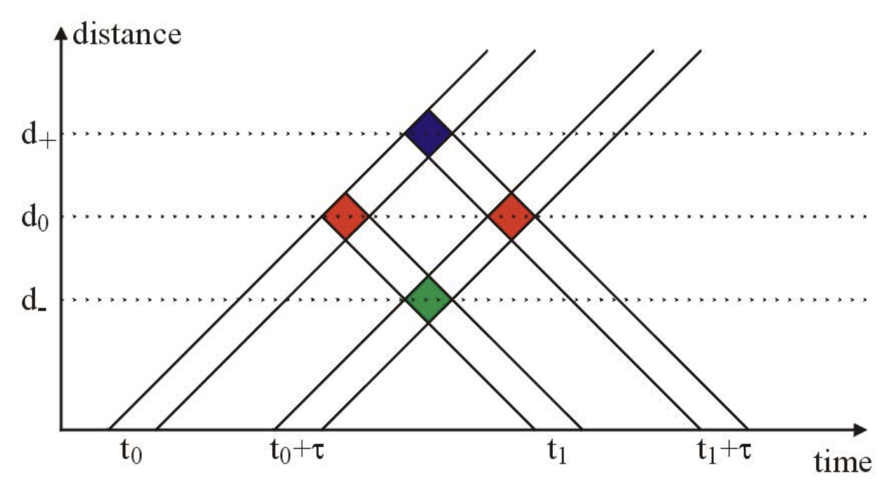
Example of a two pulse sequence with single lag and the distance of the volumes in the ionosphere that the pulse probes. Credit: K. McWilliams

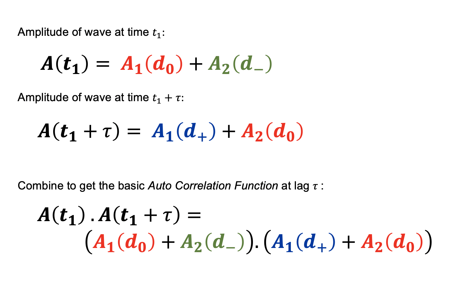
Combining the two amplitudes from the two time points, we can compare how the waves have changed, (this is called an auto-correlation function) as you are comparing it with itself but at a small single time lag of τ. We then want to remove as much of the return signals from different distances in the ionosphere (the blue and green volumes), to do this we send many 2 pulse sequences and average over all their return signals with the same lag of τ.

More Pulses?

At SuperDARN, to get the highest quality data we want to achieve this value for as many lags as possible, where a lag is any integer multiple of the original τ value. Simply adding in one more pulse which is sent at time t₀+ 3τ, to make a 3-pulse sequence, we find that we can now build a lag table of 3 different lag values.

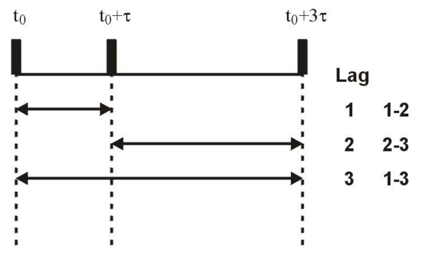
Lag table for 3-pulse sequence. Credit: K. McWilliams

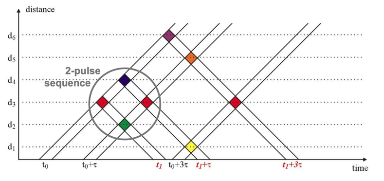
Example of a three pulse sequence with three unique lags and the distance of the volumes in the ionosphere that the pulse probes. Credit: K. McWilliams

In reality, SuperDARN radars use 7-, 8-, and 9- pulse sequences which build a lag table of up to 20+ lags. You can see what that lag table would look like on our Build Your Own Borealis Experiment tool.

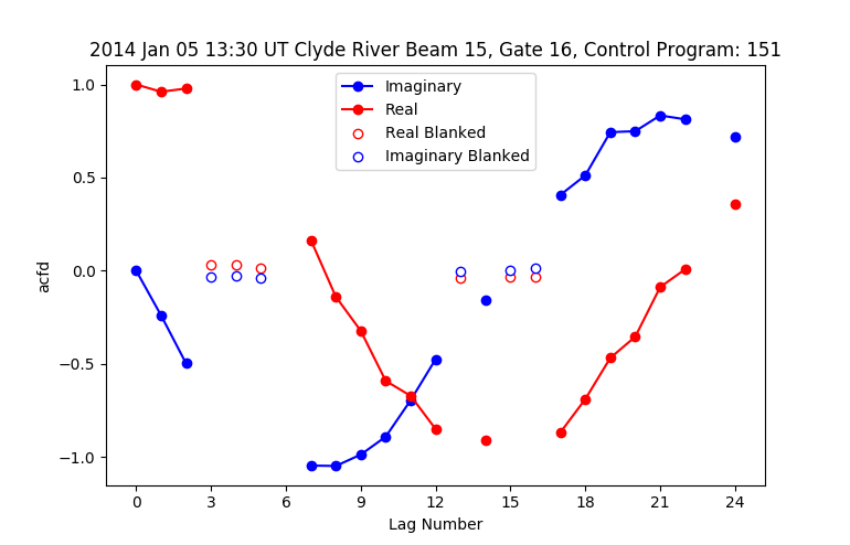
We then plot each value of the average amplitude for each lag against the lag number to produce an autocorrelation function. This is done for every range gate along the beam. The range gate is determined by the length of the pulse, generally the range gates are around 45 km, which is 300 microseconds for a single pulse. You can view real ACF data using the plotting library pyDARN, right is an example ACF from 2018.

At the speed of light, a radio wave will travel 90 km in 300 microseconds, which is 45 km there and back.

Blanked lags are either lags at which data was not retrievable (i.e. too much overlap, don't know which pulse the data originated from) or the lag table did not allow for the lag. The autocorrelation function has real and imaginary parts, the real part is the amplitude that is in phase and the imaginary part is the amplitude that is 90 degrees out of phase.

Scientific Data

Typical layout of a SuperDARN radar. From Shepherd (2017)

After all of this processing and extracting of data, we are left with a couple of data products. From the autocorrelation function, we can extract the line of sight (doppler) velocity by fitting a tangent function to the phase angle (difference in angle) between the real and imaginary parts of the autocorrelation function. Line of sight velocity means the velocity of ions only in the direction along the beam towards or away from the radar. The signal to noise ratio and the spectral width can also be calculated by fitting a Lorentzian function (which looks like a single peak) to the amplitude of the ACF.

The spectral width is a description of how long a signal persists in the same form. For example, a signal scattering off the ground will look the same for a long time, but an area of the ionosphere is always changing so will have a larger spectral width. Scatter which is from the ground and not the ionosphere can be identified by very low velocity with narrow spectral width and high power - we can then filter out this as we wish. In our real time displays the ground scatter is shown as a dark grey colour.

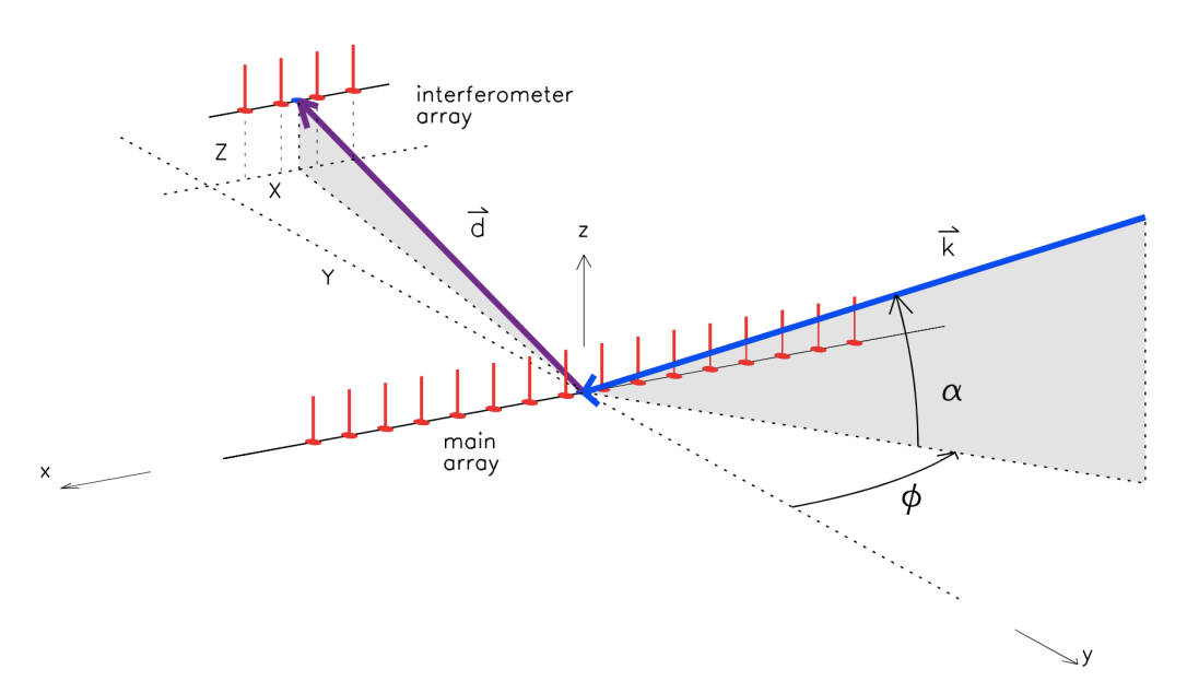
The final important variable shown in our real time displays and plots, is the elevation angle. This is more complicated to calculate. In addition to our 16 radar towers, most SuperDARN Radars also have an interferometer array. This array is an additional four radar towers set behind the main array by around 100 meters. Using this additional array we can find the angle at which the incoming radio wave is approaching the array at. This angle is used to calculate the range and altitude of the region which is returning the radio signal. And that's how we get the four main parameters seen in our real-time display.

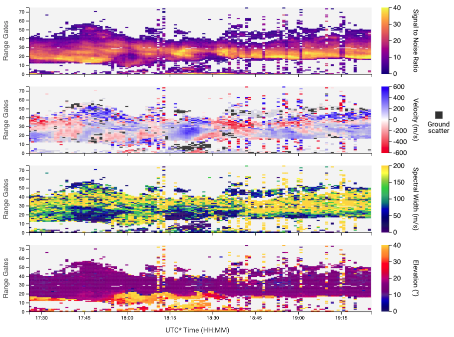
Example of real-time data for Clyde River on 29th Nov 2021.

This process of receiving a signal, processing the raw data into an ACF, then into scientific data is happening for every range-gate, on every beam for over 30 radars simultaneously, 24 hours a day and 7 days a week. And we can get that data to your computer screen in only a few seconds after the signal was being bounced off ionospheric irregularities.

SuperDARN Canada is in charge of only 5 Canadian radars, so this is a huge international project spanning nearly 30 years. The end goal of taking and processing all of this data in our ionosphere is to better understand the dynamics of our ionosphere and the effects of space weather on the human race. Once we combine data from all radars in the northern an southern hemisphere, we can make a convection map.

Convection maps shown the entire northern or southern hemisphere, overlapping fields of view from a large number of radars allow for a true vector velocity to be calculated from the single radar line of sight velocities. Combining all this, we can produce a map of how the entire ionosphere is moving in 2 minute intervals. We can see where the ionosphere is moving with Earth's magnetic field lines (Earth's Magnetosphere tutorial) in the Dungey Cycle and we can also monitor how large space weather events (Space Weather Impacts tutorial) effect us on Earth through our ionosphere.

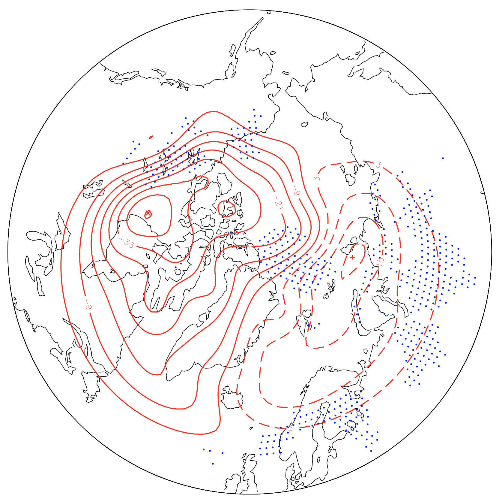
Convection map showing a typical 2 cell pattern where the ionosphere is moving from day side to night side through the middle and back around. You are looking down from above at Earth's northern hemisphere where the Sun would be off the top of the plot. Dots show where measured velocities were found from the radars. Stream lines show movement of plasma much like a weather report on wind, these stream lines are fitted using a model from the velocities.

References and Further Reading

Tutorials Home